What IS a Function?
The single most common beginner mistake: assuming functions are about numbers. They're about mappings — from anything, to anything.
The first mistake
Almost everyone arrives at “function” already carrying a picture from school: , a graph, a curve on graph paper. That picture isn’t wrong, but it’s a single special case wearing the whole concept’s name — and it quietly teaches the wrong lesson, which is that a function is fundamentally about numbers.
“A function takes a number and returns a number.” This is the single most common assumption that trips up beginners moving from math class into Functional Programming — and it’s simply false. A function is a mapping between any two sets. The inputs and outputs can be numbers, but they can just as easily be fruit, colours, people, files, or other functions.
The actual definition
A function from a set to a set is a rule that assigns to every element of exactly one element of . That’s the whole definition. Nothing in it mentions arithmetic.
- is called the domain — the set of allowed inputs.
- is called the codomain — the set the outputs are drawn from (not necessarily all of it — see below).
- The range (or image) is the subset of that actually gets hit by some input. The range is always a subset of the codomain, and sometimes a strictly smaller one.
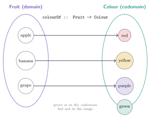
Figure: colourOf :: Fruit -> Colour. The domain is a set of fruit, the codomain a set of colours — and notice green sits in the codomain but is never actually produced, so it isn’t in the range.
In Haskell, this is written directly as a type signature:
data Fruit  = Apple | Banana | Grape
data Colour = Red | Yellow | Purple | Green

colourOf :: Fruit -> Colour
colourOf Apple  = Red
colourOf Banana = Yellow
colourOf Grape  = Purple
No numbers appear anywhere. colourOf is exactly as much a function as is — arguably a cleaner example, because there’s no temptation to think “function” means “formula you plug a number into.”
The word “function” itself comes from Leibniz, who used it around 1673 for a quantity that depends on a curve. It took another 150+ years — through Euler, Dirichlet, and eventually set theory — for the definition to loosen into the fully general “any mapping between sets” version Haskell inherits today.
Total functions vs. partial functions
Look again at the definition: every element of the domain must map to exactly one output. A function that satisfies this for its entire stated domain is called total. A function that doesn’t — one that’s undefined for some inputs — is called partial.
-- total: every list, including [], produces an answer
safeHead :: [a] -> Maybe a
safeHead []     = Nothing
safeHead (x:_)  = Just x

-- partial: crashes on []; not actually a function over ALL of [a]
head :: [a] -> a
head (x:_) = x
-- head [] ⇒ *** Exception: Prelude.head: empty list
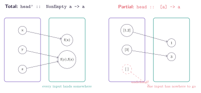
Figure: head' handles every possible NonEmpty a, so it’s total on its stated domain. The library head is only defined for non-empty lists, but its type claims to accept [a] — including [] — which is where the partiality hides.
This distinction matters enormously in Haskell, because the type signature is a promise. head :: [a] -> a promises an a for any [a] you hand it — a promise the empty list breaks at runtime. safeHead :: [a] -> Maybe a makes an honest, keepable promise instead: “you’ll get something, but that something might be ‘nothing.’” Preferring total functions — functions whose types tell the truth about every input — is one of the most valuable habits Haskell teaches.
An ordinary Haskell function a -> b is total by convention (ignoring undefined and infinite loops, which theorists call “bottom,” written ). A genuinely partial function is instead usually modeled as a total function into Maybe b — turning “sometimes has no answer” into an honest value, Nothing, that lives in the codomain. This is the first hint of a pattern this book returns to again and again: Haskell tends to make partiality, failure, and effects into values, rather than exceptions to the rules.
Injective, surjective, bijective: three useful shapes
Total and partial describe whether a function is fully defined. A second, independent question — one about the shape of the mapping itself — turns out to matter just as much in practice: does the function ever collide two different inputs onto the same output, and does it ever leave part of the codomain untouched?
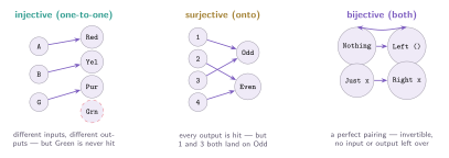
Figure: colourOf from earlier in this chapter is genuinely injective — no two fruits share a colour — but not surjective, since Green sits in the codomain unreached. A function can be one, the other, both, or neither.
Injective (“one-to-one”) means different inputs always produce different outputs:
-- injective: no two distinct Ints ever produce the same Integer
widen :: Int -> Integer
widen = fromIntegral
Surjective (“onto”) means every element of the codomain gets hit by some input — the range equals the whole codomain, with nothing left over:
colourOf from earlier is not surjective onto Colour, since Green is never produced — exactly the gap the figure above illustrates between codomain and range.
Bijective means both at once — a perfect pairing between domain and codomain, with nothing missed and nothing doubled up:
data Direction = North | East | South | West deriving (Show, Eq, Enum, Bounded)

toIndex :: Direction -> Int
toIndex = fromEnum

fromIndex :: Int -> Direction
fromIndex = toEnum

-- fromIndex . toIndex === id, and toIndex . fromIndex === id (on 0..3)
Bijective functions are exactly the ones with a genuine, well-defined inverse — toIndex and fromIndex undo each other exactly, which is proof that Direction and {0, 1, 2, 3} are, structurally, the same shape wearing different names — an isomorphism, the same word and the same idea this book reaches for again once Zippers and Derivatives shows two very differently-described types turning out to be identical underneath.
This classification matters practically, not just theoretically: a bijection is exactly the condition under which toEnum/fromEnum round-trip safely, and it’s the condition a JSON encoder/decoder pair, or a database schema migration, needs to satisfy to guarantee no information is silently lost or duplicated in either direction.
It’s tempting to assume a function and its “inverse-shaped” counterpart are automatically inverses of each other just because their types line up — Show’s show and Read’s read are the classic trap. show is total and (for well-behaved types) injective, but read . show only round-trips correctly if read’s input is exactly what show would have produced; hand it slightly different formatting and read can fail outright, meaning read isn’t a true, total inverse of show the way fromIndex is a true inverse of toIndex above.
Functions are values too
One more habit worth building early: in Haskell, a function is not a special kind of thing separate from “data” — it’s a value like any other, and can be passed around, stored, and returned from other functions.
apply :: (a -> b) -> a -> b
apply f x = f x

twice :: (a -> a) -> a -> a
twice f = f . f

-- colourOf itself, unapplied, is a perfectly ordinary value:
lookupTable :: [Fruit -> Colour]
lookupTable = [colourOf, colourOf]
This is what people mean by “functions are first-class” — and it’s the property that makes everything from Chapter 9 onward (fmap, <*>, >>=) possible: they’re just ordinary functions that happen to take other functions as arguments.
Closures: a function that remembers where it came from
Being a first-class value gets more interesting the moment a function returns another function:
makeAdder :: Int -> (Int -> Int)
makeAdder n = \x -> x + n

addFive :: Int -> Int
addFive = makeAdder 5

ghci> addFive 10
15
makeAdder 5 doesn’t just compute a number — it builds a brand-new function, \x -> x + n, with n already fixed at 5. That returned function keeps carrying 5 around with it, long after makeAdder itself has finished running and its local n would otherwise be gone. This bundle — a function paired with the values it captured from the scope it was born in — is called a closure.
The term itself is exactly as old as the field’s attempt to take this idea seriously. Peter Landin — the same Landin behind ISWIM and Base Camp’s own history section — coined “closure” in his 1964 paper “The Mechanical Evaluation of Expressions,” describing it precisely as a lambda expression bundled with the environment needed to make sense of it. The problem closures solve had already embarrassed Lisp for years before Landin named it: Lisp’s original dynamic scoping meant a function returned from another function could see the wrong variables — whatever happened to be in scope at the call site, not at the function’s own birthplace — a bug serious enough that Joel Moses’s 1970 MIT paper diagnosing it was literally titled “Why the FUNARG Problem Should Be Called the Environment Problem.” Guy Steele and Gerald Sussman adopted Landin’s term directly when they built proper lexical scoping into Scheme in 1975 — the same Scheme already covered in Base Camp’s own timeline.
Closures took a strikingly long time to reach the languages most working programmers actually used. C never got them at all — a C function pointer can be passed around freely, but it captures no environment whatsoever; there is simply no n for it to remember. Java’s workaround, anonymous inner classes, remained the only option for nearly two decades, until Java 8 (2014) finally added real lambda expressions — with one lingering, very deliberate restriction: a Java lambda can only capture a local variable that’s effectively final (never reassigned after its first value), and it captures that variable’s value at closure-creation time, not the variable itself. JavaScript’s closures, by contrast, capture the actual mutable variable, exactly the way Haskell’s would if Haskell had mutable variables to capture — which is precisely why “Java lambdas aren’t quite true closures” is a real, commonly-made distinction, not pedantry.
Implementing the classics: map, filter, and friends
“Functions as values” stops being an abstract slogan the moment you see it used constantly, in code you’d write on any ordinary day. Four of the most common list functions in Haskell — map, filter, take, takeWhile — are themselves nothing more than ordinary recursive functions that happen to take a function as one of their arguments. Seeing their actual definitions is worth more than any amount of description:
map' :: (a -> b) -> [a] -> [b]
map' _ []     = []
map' f (x:xs) = f x : map' f xs

filter' :: (a -> Bool) -> [a] -> [a]
filter' _ []     = []
filter' p (x:xs)
  | p x       = x : filter' p xs
  | otherwise = filter' p xs
map' walks the list, applying f to every element and keeping every result — the output is always exactly as long as the input. filter' walks the same way, but only keeps an element when the predicate p approves it — the output can be any length from zero up to the input’s length, depending entirely on how many elements pass.
take' :: Int -> [a] -> [a]
take' n _ | n <= 0 = []
take' _ []         = []
take' n (x:xs)     = x : take' (n - 1) xs

takeWhile' :: (a -> Bool) -> [a] -> [a]
takeWhile' _ []     = []
takeWhile' p (x:xs)
  | p x       = x : takeWhile' p xs
  | otherwise = []

ghci> take' 3 [1,2,3,4,5]
[1,2,3]
ghci> takeWhile' (< 5) [1,2,3,7,2,1]
[1,2,3]
ghci> filter' (< 5) [1,2,3,7,2,1]
[1,2,3,2,1]
take' and takeWhile' look like close cousins of filter', but the distinction between the last two is worth sitting with: filter' scans the entire list and keeps every element that passes, however far apart they are, while takeWhile' stops at the first failure and never looks any further, even if elements further along would have passed too. takeWhile' (< 5) [1,2,3,7,2,1] gives [1,2,3] — the 2 and 1 after the 7 are never even examined, let alone kept — while filter' (< 5) on the identical list keeps them, giving [1,2,3,2,1]. Reaching for the wrong one of these two is a classic, easy-to-miss bug.
Lambda expressions (Base Camp) are what make calling any of these feel natural without first writing a separate named helper:
ghci> map' (\x -> x * x) [1,2,3,4]
[1,4,9,16]
ghci> filter' (\x -> x `mod` 3 == 0) [1..15]
[3,6,9,12,15]
\x -> x * x is a function exactly like colourOf or square — it just never got a top-level name, because it’s only ever going to be used once, right here, as map'’s argument. Once a lambda like this becomes familiar enough to read at a glance, it’s often rewritten point-free (Chapter 2) instead — map' (\x -> x * x) xs and map' (^2) xs compute the identical thing, and choosing between them is purely a readability call, not a correctness one.
The real Prelude versions of map, filter, take, and takeWhile behave identically to the ones above but are written to work lazily and efficiently over Haskell’s actual list representation — the hand-written versions here are chosen for clarity, not performance, exactly the same “clarity first” instinct Pearls built its entire chapter around.
Composing functions: the algebra underneath
(.), already used silently since Chapter 2’s point-free style section, is itself worth a formal look — because the shape it has turns out to be an exact instance of the Monoid chapter’s own pattern, not just a loose analogy to it.
(.) :: (b -> c) -> (a -> b) -> (a -> c)
(f . g) x = f (g x)
Composition satisfies both a Monoid’s laws, for functions of type a -> a specifically. It’s associative: (f . g) . h and f . (g . h) always compute the identical function, for any f, g, h — exactly Monoids’ associativity law, one level up, combining functions instead of values. And it has an identity element: id, the function that returns its argument unchanged, satisfies id . f = f = f . id for every f — precisely mempty’s role, played by a function instead of a value.
newtype Endo a = Endo { appEndo :: a -> a }

instance Semigroup (Endo a) where
  Endo f <> Endo g = Endo (f . g)

instance Monoid (Endo a) where
  mempty = Endo id
Data.Monoid.Endo is exactly this — a real, standard-library newtype wrapper making the observation official: functions from a type to itself, under composition, are a Monoid, with (.) playing <> and id playing mempty. This isn’t a cute parallel invented for this book; it’s the literal instance declaration, sitting in base, that any Haskell program can import and use.
mconcat (Monoids) on a list of Endo-wrapped functions gives you function composition applied to an entire list at once — appEndo (mconcat (map Endo [(+1), (*2), subtract 3])) builds the pipeline (+1) . (*2) . subtract 3 automatically, purely because Endo’s Monoid instance already knows how to fold a list of functions down to one, the exact same foldr (<>) mempty shape every other Monoid in this book has used.
Try it yourself
square :: Integer -> Integer
square x = x * x
Here the domain is (all integers), the codomain is (non-negative integers — Haskell’s Integer doesn’t enforce this, but mathematically that’s the honest codomain), and the range is the even smaller set of perfect squares . Three different sets, three different roles — and not one of them requires you to imagine a graph.