The Runtime System and Performance Tooling
Every warning this book has given about thunk buildup and space leaks has been a claim about what happens at runtime — this chapter is how to stop taking those claims on faith and actually watch the runtime system prove or disprove them.
The RTS: what’s actually running your program
Every compiled Haskell executable carries something most languages keep entirely invisible: the RTS, GHC’s runtime system — a garbage collector, a lightweight-thread scheduler (Beautiful Concurrency’s green threads are RTS machinery), and memory management, all linked directly into the binary. Unlike most compiler flags, RTS behavior can be tuned after compilation, at the moment the program actually runs, using +RTS ... -RTS:
./myprogram +RTS -s -RTS
-s alone is worth building a habit around — it prints a summary of exactly what the RTS did, after the program exits:
   1,234,567,890 bytes allocated in the heap
      45,678,901 bytes copied during GC
          12,345 bytes maximum residency
              23 MB total memory in use

  Generation 0:    89 collections,     0 parallel
  Generation 1:     4 collections,     0 parallel

  INIT    time    0.001s
  MUT     time    0.245s
  GC      time    0.032s
  Total   time    0.278s
“Bytes allocated” is often startlingly larger than a program’s actual data — Haskell allocates constantly, for every thunk, every cons cell, every intermediate value, and relies entirely on the garbage collector reclaiming most of it almost immediately. “Maximum residency” — the peak amount the GC couldn’t reclaim at any single point — is the number that actually matters for a program’s real memory footprint, and the one worth watching for the tuple-trap-style leaks this book has warned about since Chapter 6.
Profiling: where is the time actually going?
-s answers “how much,” not “where.” For that, compile with profiling support and ask GHC to insert cost centres — bookkeeping markers attached to functions, tracking how much time and how many allocations happen inside each one:
ghc -prof -fprof-auto MyProgram.hs
./MyProgram +RTS -p
Running with -p produces a .prof file breaking down exactly where a run spent its time:
COST CENTRE   MODULE   %time   %alloc

sortBy        Main      42.1    38.7
insert        Main      31.5    29.2
member        Main      18.9    22.4
-fprof-auto inserts a cost centre at nearly every function boundary automatically — convenient for a first pass, though it can distort the numbers slightly by adding overhead of its own; hand-placed cost centres ({-# SCC "expensive-part" #-}) on just the functions actually under suspicion give a more surgical picture once the first profile has narrowed down where to look.
Heap profiling: watching thunks pile up, literally
Time profiling answers “what’s slow.” Heap profiling answers the question this book’s entire Laziness and Practical Haskell chapters have been building toward: “is something quietly holding onto memory it should have let go of?”
ghc -prof -fprof-auto MyProgram.hs
./MyProgram +RTS -hc          # heap profile, grouped by cost centre
hp2ps -c MyProgram.hp          # render the .hp file to a PostScript graph
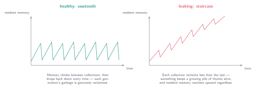
Figure: A healthy sawtooth heap profile versus a leaking staircase — the same shape this book’s space-leak warnings have been describing in words, now something you can actually watch happen.
A healthy program’s heap profile looks like a sawtooth: memory climbs as thunks and intermediate values accumulate between garbage collections, then drops sharply every time the collector runs and reclaims what’s actually dead. A leaking program’s profile instead climbs in a staircase — each collection reclaims less than the last, because something (Practical Haskell’s tuple trap is the canonical example) is keeping a growing chain of thunks reachable, so the collector has less and less genuinely-dead memory to find each time it runs.
-hc groups the heap by cost centre — useful for “which function’s data is piling up,” but it won’t tell you why that data is still reachable. -hy (group by type) and -hd (group by closure description, showing actual unevaluated thunks by name) are the sharper tools once -hc has pointed at a suspect function — reach for the coarser view first, then narrow.
Benchmarking properly: Criterion
-s’s wall-clock time is a single, noisy measurement — enough to notice something is slow, not nearly rigorous enough to trust a 5% improvement claim. Criterion, the standard Haskell microbenchmarking library, runs a benchmark enough times to build a real statistical picture — mean, standard deviation, outlier detection — rather than reporting one lucky (or unlucky) run. A realistic benchmark suite usually compares more than two candidates at once, and shares expensive setup between them with env:
import Criterion.Main
import qualified Data.List as List

main :: IO ()
main = defaultMain
  [ env (pure (reverse [1..5000 :: Int])) $ \testData ->
      bgroup "sorting 5000 elements"
        [ bench "insertion sort" $ nf insertionSort testData
        , bench "merge sort"     $ nf mergeSort testData
        , bench "Data.List.sort" $ nf List.sort testData
        ]
  ]
benchmarking sorting 5000 elements/insertion sort
time                 48.32 ms   (47.91 ms .. 48.77 ms)
                     0.999 R²

benchmarking sorting 5000 elements/merge sort
time                 3.104 ms   (3.089 ms .. 3.121 ms)
                     0.998 R²

benchmarking sorting 5000 elements/Data.List.sort
time                 2.187 ms   (2.171 ms .. 2.203 ms)
                     0.999 R²
env builds testData exactly once, shared across all three benchmarks in the group, so the cost of constructing the test input never contaminates any individual timing — without it, the setup cost would silently get folded into whichever benchmark happened to force it first. Running the compiled benchmark executable with --output report.html produces an interactive HTML report with real graphs (a kernel density estimate of the timing distribution, not just a single number) — genuinely worth generating the first time a benchmark result needs to be shared with, or defended to, someone else.
nf (normal form — Laziness’s own vocabulary) forces the entire result before timing stops, avoiding the classic mistake of accidentally benchmarking how long it takes to build an unevaluated thunk rather than the actual computation. This is exactly the tool for Pearls’ and Common Algorithms’ “clarity first, measure before optimizing” instinct put into practice — a real, repeatable number, rather than a guess about which of two implementations is actually faster. (For what it’s worth: Data.List.sort wins here for exactly the reasons Common Algorithms’ own chapter would predict — it’s a real, tuned merge sort implementation, benefiting from years of low-level optimization the hand-written version above was never trying to compete with.)
Criterion doesn’t just run a benchmark times and average — it uses linear regression across multiple different iteration counts to separate a benchmark’s genuine per-iteration cost from fixed overhead (JIT-style warmup doesn’t apply to compiled Haskell, but OS scheduling noise and cache effects very much do), which is why its output includes an goodness-of-fit statistic alongside the timing itself: a low is Criterion’s own way of warning that a result is noisier than it looks.
Seeing what the CPU actually did: perf
Criterion answers “how long,” rigorously. It can’t answer “why” at the hardware level — how many instructions actually ran, how often a cache was missed, how often a branch was mispredicted. perf, Linux’s own system-wide profiler, sees exactly that, for any compiled binary — it has no idea a program is written in Haskell at all, and that’s precisely what makes it a useful complement to GHC’s own cost-centre profiler rather than a replacement for it.
ghc -O2 -g Sorts.hs -o sorts    # -g: emit debug info perf can read
perf stat ./sorts
 Performance counter stats for './sorts':

        128.45 msec task-clock                #    0.998 CPUs utilized
             3       context-switches          #   23.36  /sec
             0       cpu-migrations            #    0.00  /sec
         1,204       page-faults               #    9.37 K/sec
   412,384,921       cycles                    #    3.21 GHz
   891,234,567       instructions              #    2.16  insn per cycle
   178,234,012       branches                  # 1387.45 M/sec
     2,341,201       branch-misses             #    1.31% of all branches

       0.128721466 seconds time elapsed
-g tells GHC to emit DWARF debug information, so perf can report actual Haskell function names in its output rather than raw memory addresses. perf stat gives a quick hardware-level summary in one shot — “instructions per cycle” (IPC) above 2 is generally healthy; a program with a surprisingly low IPC despite looking algorithmically fine is a strong hint that cache misses or branch mispredictions, not the algorithm itself, are the actual bottleneck. perf record -g ./sorts followed by perf report goes further, producing an interactive, sorted-by-percentage breakdown of exactly which functions — including inside GHC’s own runtime and garbage collector, invisible to -p’s cost centres — consumed the most CPU time.
GHC’s own -p profiler and perf answer genuinely different questions, and conflating them is a common mistake: -p shows logical cost — which Haskell function, by name, according to the cost centres this chapter’s earlier section inserted — while perf shows physical cost, at the level of actual machine instructions, including time spent inside the RTS and garbage collector that never shows up as a Haskell cost centre at all. A function that looks cheap under -p can still be the actual hardware bottleneck, if the real cost is GC pressure it indirectly causes rather than time spent in the function’s own body.
Watching concurrency: ThreadScope
Beautiful Concurrency’s green threads and STM transactions are, at runtime, genuinely concurrent activity — and ThreadScope is the tool for watching that activity happen, rather than reasoning about it purely on paper:
ghc -eventlog MyProgram.hs
./MyProgram +RTS -ls -N4    # -N4: use 4 OS threads; -ls: log scheduler events
threadscope MyProgram.eventlog
The resulting timeline shows every green thread’s activity across each OS thread over time — genuinely useful for spotting a common, otherwise-invisible problem: a program compiled with -N4 that never actually uses more than one core at once, because its workload wasn’t structured to give the scheduler real parallel work to do.
Production Haskell services commonly ship with -s (or the machine-readable --machine-readable variant) enabled by default in their deployment configuration, feeding GC statistics straight into monitoring dashboards alongside ordinary application metrics — a staircase-shaped resident-memory graph in production is treated exactly as seriously as an error rate spike, and for the same reason: it means something is systematically wrong, not just occasionally slow.
Every diagnostic in this chapter answers a question this book has, until now, only ever answered in prose: is this thunk actually being forced when expected, is this data actually being reclaimed, is this algorithm actually faster in practice. The RTS doesn’t change any of the reasoning from earlier chapters — it’s the same laziness, the same strictness, the same WHNF this book has built up from Chapter 6 onward — but it turns “should be” into something you can point a tool at and check.