Lambda Calculus: The Engine Underneath
Before there was Haskell, before there were computers at all, Alonzo Church wrote down a system with three rules that turned out to be able to compute anything computable. Every function you will ever write in Haskell is that system, wearing nicer syntax.
What even is a “lambda,” and what even is a “calculus”?
Both halves of this chapter’s name are easy to misread. “Calculus” makes almost everyone think of derivatives and integrals — the calculus taught in school — but that’s just one particular calculus. In mathematics and logic more broadly, “a calculus” means something much more general: any formal system for calculating by symbolic manipulation, following fixed rules, with no reference to what the symbols “mean.” Propositional calculus, sequent calculus, and Church’s lambda calculus are all calculi in this older, broader sense — the family resemblance is “rules for manipulating symbols,” not “rates of change.” Lambda calculus has nothing to do with slopes or areas under curves; it’s a calculus the way “calculus” meant, originally, before Newton and Leibniz’s version became the one everyone learns first.
“Lambda” is just the Greek letter Church picked to write “here’s a function” — but why that particular letter is a genuinely unresolved, and genuinely funny, piece of history.
The leading theory, traced by historians Cardone and Hindley through Church’s own student J. Barkley Rosser, is pure typesetting accident: Whitehead and Russell’s Principia Mathematica wrote “the class of all x such that f(x)” with a caret over the x, like . Church, needing a similar but distinct notation for function abstraction rather than class abstraction, moved the caret to sit just left of the x instead of above it. A typesetter, apparently unable to position the mark cleanly, gave it a small tail — and the tailed caret gradually became a lambda. But Church himself muddied this story later in life: in a 1964 letter, and again when asked directly by at least two later correspondents why he’d chosen lambda specifically, he described the choice as essentially arbitrary — a symbol was needed, and this one was picked. Even the man who invented it gave two different, equally plausible answers to where it came from.
A calculus with nothing in it but functions
In 1936, Alonzo Church was trying to formalize what it means for something to be “effectively computable” — decades before any electronic computer existed to compute anything. His answer, the lambda calculus, is almost shocking in how little it contains. There are no numbers, no booleans, no lists, no built-in arithmetic. There is exactly one kind of thing — the function — and exactly three rules for building and manipulating them.
That’s it. And it turns out to be exactly as powerful as a Turing machine: anything one can compute, the other can too. Haskell is, in a very real sense, the lambda calculus with pockets sewn in — the same three rules underneath, plus types, syntax, and a standard library layered on top for convenience.
The three pieces
A term in the lambda calculus is built from just three things:
- Variables —
x,y,z, … - Abstraction —
λx. e, a function that takes an argument calledxand returns the expressione - Application —
e1 e2, applying the functione1to the argumente2
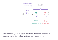
Figure: λx. (x y), taken apart. The λx. is the abstraction — it binds x for the rest of the term. Everything after the dot is the body. Inside the body, x is a bound occurrence (it refers back to the abstraction), while y is free — it isn’t bound by anything in this term at all.
Translate this directly into Haskell and nothing is lost:
-- λx. x + 1        becomes:
\x -> x + 1

-- λx. λy. x + y    becomes (a function returning a function):
\x -> \y -> x + y
That second example is worth sitting with. λx. λy. x + y is a function of one argument, x, that returns another function, which itself takes y and returns x + y. There is no such thing as a genuinely two-argument function in the lambda calculus — only functions that return functions. Haskell’s \x y -> x + y and multi-argument type signatures like (->) :: a -> b -> c are sugar over exactly this: currying, named after Haskell Curry, is built into the calculus at its foundation, not bolted on as a Haskell-specific feature.
It’s tempting to read f :: Int -> Int -> Int as “a function of two Ints.” More precisely, it’s a function of one Int that returns a function Int -> Int. This isn’t pedantry — it’s what makes partial application (add5 = (+) 5) work at all: you’re just applying the outer function and stopping before you supply the second argument.
The one computation rule: beta reduction
The lambda calculus has exactly one rule for actually computing anything: beta reduction. When a function meets its argument, you substitute the argument for every free occurrence of the bound variable in the body.
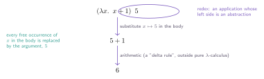
Figure: (λx. x + 1) 5 is a redex — a “reducible expression,” an application whose left side is an abstraction. Beta reduction substitutes 5 for x throughout the body, giving 5 + 1; a further arithmetic step (technically outside the pure calculus, added back in as a convenience) gives 6.
That single substitution rule, applied over and over, is the entire computational engine — not just of the lambda calculus, but underneath every let, every function call, every pattern match Haskell ever performs. When GHC evaluates (\x -> x + 1) 5, it is doing beta reduction, full stop.
Substituting carefully: alpha-conversion
Substitution has to be done with real care, or it silently breaks. Consider λy. (λx. λy. x y) y — substituting the free y from outside into the inner λx. λy. x y:
λy. (λx. λy. x y) y
  →  (naive substitution: replace x with y)
λy. (λy. y y)
Something has gone wrong. The outer y — the one the substitution was supposed to carry in — has been silently captured by the inner λy., which rebinds the name y before the substituted value ever gets used. The inner λy. y y no longer refers to the outer y at all; it’s a completely different function now, one that ignores its argument’s origin entirely. This is variable capture, and it’s exactly the kind of bug that would make substitution — the calculus’s only computation rule — silently produce the wrong answer.
The fix is alpha-conversion: bound variables can always be systematically renamed without changing a term’s meaning (λx. x and λz. z are the same function), so before substituting, rename the inner λy. to something guaranteed not to collide:
λy. (λx. λz. x z) y     -- inner y renamed to z first, harmlessly
  →  (now substitute x with y — no collision possible)
λy. (λz. y z)
The renamed version correctly preserves the outer y’s identity all the way through. GHC’s compiler internals handle exactly this kind of hygiene automatically, every time it inlines or specializes your code — the reason Haskell programmers essentially never think about variable capture, despite it being a genuine, sharp edge of the underlying calculus, is that alpha-conversion is applied silently, correctly, and constantly underneath.
Combinators and point-free style
Look back at that variable-capture warning for a moment. It’s only a concern because λy. x has a free variable — x isn’t bound by anything inside the term itself; its meaning depends on whatever surrounds it. A term with no free variables at all — one that is entirely self-contained — is called a combinator, and combinators turn out to be worth naming individually, because a small handful of them show up constantly.
identity = \x -> x               -- traditionally called I
konst    = \x -> \y -> x         -- traditionally called K
subst    = \x -> \y -> \z -> x z (y z)   -- traditionally called S
I, K, and S are the three combinators of SKI combinator calculus, a system Moses Schönfinkel and Haskell Curry showed in the 1920s and 30s can express everything the full lambda calculus can — variables and all — using nothing but these three closed terms and application. K is worth sitting with: K x y = x throws its second argument away entirely and returns the first, unconditionally — which is exactly the shape of “ignore this, keep that.”
I and K aren’t just historical curiosities — they’re sitting in the Haskell standard library under more ordinary names. id :: a -> a is I, verbatim. const :: a -> b -> a is K, verbatim: const x _ = x throws away its second argument exactly the way K does. Even S has a living relative: Control.Monad’s ap and Applicative’s <*> (Chapter 10) generalize S’s “apply, but thread an extra argument through both sides” shape from plain functions to any applicative context.
Combinators earn their name because they combine their arguments — rearranging, duplicating, or discarding them — without ever needing to look anything up in a surrounding environment. That self-containedness is precisely what makes point-free style possible: writing a function definition without ever naming the argument it’s applied to.
-- "pointful": x is named, and appears explicitly
sumOfSquares :: [Int] -> Int
sumOfSquares xs = sum (map (^2) xs)

-- point-free: no argument is ever named
sumOfSquares' :: [Int] -> Int
sumOfSquares' = sum . map (^2)
Here, “point” is used in its mathematical sense — a specific input value — not a typo for “pointer.” sumOfSquares' is defined purely by composing two existing functions, sum and map (^2), with (.), rather than by naming an xs and describing what happens to it. The list argument is still there, implicitly — sumOfSquares' still has type [Int] -> Int — it simply never needs a name, because the definition is built entirely out of combinators ((.) itself is a combinator, traditionally called B) gluing other functions together.
Point-free style is a satisfying puzzle to write, but it is not automatically clearer — a long chain of composed combinators with no named intermediate values can just as easily become a genuinely harder read than the pointful version, especially once more than two or three functions are chained together. Haskell programmers generally reach for point-free style when it reads like a natural pipeline (sort . nub . map toLower), and drop back to naming arguments the moment doing so would actually aid understanding. Being able to eliminate every point is not the same as should.
The rule that justifies it: eta-conversion
Beta reduction and alpha-conversion aren’t the calculus’s only rules — there’s a third, quieter one that’s exactly what makes point-free style legitimate rather than just a lucky syntactic trick. Eta-conversion says that λx. f x and f itself are the same function, for any f that doesn’t already mention x:
-- eta-expanded: x is named, applied immediately, and thrown away
increment :: Int -> Int
increment = \x -> succ x

-- eta-reduced: the same function, with the redundant wrapper removed
increment' :: Int -> Int
increment' = succ
Both versions behave identically for every possible input, because applying either one to some y reduces to succ y either way — the \x -> ... x wrapper genuinely adds nothing beyond a name that’s immediately used once and discarded. This is precisely the justification for the point-free rewrites above: sumOfSquares' = sum . map (^2) isn’t a coincidental simplification of sumOfSquares xs = sum (map (^2) xs) — it’s provably the same function, by eta-conversion, applied silently every time a trailing argument is dropped from both sides of a definition.
GHC’s own optimizer performs eta-reduction (and its reverse, eta-expansion) routinely and automatically while compiling — sometimes expanding a point-free definition back out internally, because the expanded form occasionally allows other optimizations to fire that the compressed form would hide. The rewrite you write and the code GHC actually runs are related by exactly these three rules — alpha, beta, eta — applied far more times, and far more mechanically, than any human would want to trace by hand.
From untyped to Haskell
The system above — the untyped lambda calculus — is what Church actually wrote down, and it’s powerful enough that some terms (\x -> x x, applying a function to itself) typecheck in no sensible type system at all: x would need to be both a and a -> b simultaneously. Haskell is built on the simply-typed lambda calculus instead, which adds exactly the discipline Chapter 4 described: every term gets a type, decided before anything runs, at the cost of ruling out a few things — like unrestricted self-application — that the untyped calculus permitted.
That tradeoff — a little less raw power, in exchange for the guarantee that well-typed programs can’t go wrong in certain ways — is the Curry–Howard correspondence from Chapter 4 in its native habitat: type systems and logic turn out to be the same mathematics, viewed from two directions, and the lambda calculus is the shared root both grew from.
This chapter kept things practical — just enough of the calculus to explain currying, beta reduction, and why point-free style is more than a stylistic trick. The untyped calculus has considerably more up its sleeve than what was needed here: it can build its own data out of nothing but functions, achieve recursion with no way to name anything, and its choice of evaluation order turns out to be the actual mathematical reason Haskell is lazy at all. That’s worth its own visit, once laziness itself has had a chance to earn your trust first.