Base Camp: A Whirlwind Tour of the Haskell Landscape
Type signatures, pattern matching, guards, currying, sections, lambdas, recursion — the practical vocabulary every later chapter assumes you already have. If any of this is new, start here. If none of it is, skip ahead with a clear conscience.
This chapter is a detour, not a peak. Every chapter from here on assumes you can read an ordinary Haskell function definition fluently — pattern matching, guards, sections, currying, the works. If you already can, skip straight to Chapter 2 with a clear conscience; nothing below is a prerequisite you’ll be quizzed on later. If Haskell syntax is new to you, stay a while — this is the base camp the rest of the climb is launched from.
Where this all came from
It’s worth knowing, before diving into syntax, that almost none of Haskell’s core ideas were invented for Haskell. Every major feature this book spends a chapter on — pattern matching, algebraic data types, laziness, a Hindley-Milner type system — already existed, tested and refined, in earlier languages. Haskell’s actual invention was something rarer: the discipline to combine all of them into one coherent, uncompromising language, and the restraint to say no to anything that didn’t fit.
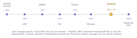
Figure: Each language solved a real problem the last one exposed — Haskell’s 1987 committee formed specifically to stop this fragmentation, unifying a decade of independently-invented lazy functional research languages into one shared standard.
Lambda Calculus (1936). Chapter 2 covers this properly, but the short version: Alonzo Church’s minimal calculus of substitution — nothing but variables, function application, and function definition — turned out to be enough to express any computable function, decades before an electronic computer existed to run one on. Every functional language since has been, in some sense, lambda calculus with better ergonomics.
LISP (1958). John McCarthy’s LISP was the first language to take functions seriously as a foundation, not just a convenience — functions as first-class values, recursion as the primary looping construct, and code itself represented as ordinary, manipulable data (the famous “code is data” idea). LISP’s parenthesized syntax has outlived nearly every contemporary from its era, but it was dynamically typed and, by modern functional standards, permissive about mutation — the strict type discipline and purity this book has spent chapters on were still decades away.
ISWIM (1966). Peter Landin’s paper “The Next 700 Programming Languages” never shipped as a real, implemented language — but it proposed something genuinely prophetic: a language built entirely around expressions rather than statements, with let and where as core constructs (both already familiar from earlier in this chapter) rather than syntactic afterthoughts. ISWIM’s central claim — that most programming languages are just minor variations on one underlying expression-oriented core — quietly shaped nearly every functional language that followed.
ML (1973). Robin Milner built ML (originally “Meta Language”) at Edinburgh, not as a general-purpose language at all, but as the scripting language for a theorem prover. Two of its ideas turned out to matter far beyond that original purpose: algebraic data types (Chapter 5’s data Shape = Circle Double | Rectangle Double Double, essentially unchanged) and Hindley-Milner type inference — the ability to work out a program’s types automatically, without the programmer writing most of them down, which is exactly why so little of this book’s Haskell code needs explicit type annotations.
Hindley-Milner inference is named for two people who discovered essentially the same algorithm independently: Roger Hindley, working on a different problem (type-checking in combinatory logic) in 1969, and Robin Milner, building ML’s type system, in 1978. Milner’s version is the one that made it into working compilers, but the underlying mathematics had already been proven sound years before any functional language actually used it.
Scheme (1975). Guy Steele and Gerald Sussman’s Scheme pared LISP back down to something closer to Church’s original lambda calculus — a small, uniform core with lexical scoping done properly, and a renewed emphasis on functions and recursion as the primary tools of the language, rather than one style choice among many.
Miranda (1985). David Turner’s Miranda is Haskell’s most direct ancestor, and the resemblance is not subtle: purity, laziness by default, a Hindley-Milner type system, and — genuinely striking to read side by side — nearly identical syntax for pattern matching, guards, where clauses, list notation, and list comprehensions. Miranda was proprietary software, though, licensed by Research Software Ltd rather than freely available — which turns out to be the single fact that explains why Haskell exists at all.
Why a committee, and why 1987
By the mid-1980s, more than a dozen different research groups had each built their own lazy, purely functional language — genuinely similar to each other in spirit, but incompatible in practice, splitting a small research community’s effort a dozen different ways with no shared platform to build on. In 1987, a committee formed with a specific, practical goal: stop the fragmentation, and standardize on one open, freely available language that captured what all of these efforts were independently converging toward. Miranda was the closest existing template — hence the strong family resemblance — but Miranda’s license meant the new language had to be its own clean implementation, not simply “open Miranda.”
The result, first released in 1990, was named Haskell, after the logician Haskell Curry — whose own work (Further Reading) is exactly where currying, used silently in nearly every function this book has written, gets its name. Language design by committee has a reputation for producing compromises nobody’s happy with; Haskell is the rare counterexample, in large part because the committee’s members were the same researchers who’d spent the previous decade building the languages Haskell unified in the first place.
The Haskell committee’s own retrospective paper — “A History of Haskell: Being Lazy with Class,” written by four of its original members in 2007 — is exactly the “committee members explain their own dead ends and compromises” read Further Reading recommends. It’s also refreshingly honest about the parts that didn’t work on the first try; monadic I/O, the entire subject of Chapter 7, took the committee several serious wrong turns before settling on the design this book teaches as though it were obvious from the start.
Haskell 98 (1998) stabilized the language into a single, documented standard — deliberately conservative, freezing a common core so textbooks, teaching materials, and multiple independent compiler implementations could all target the same target without chasing a moving specification. GHC, the Glasgow Haskell Compiler this book’s Base Camp already has you using, has been the dominant implementation since the early 1990s, and — via extensions (Chapter 17) — is also where most of the post-1998 evolution of the language actually happens; Haskell 98’s successor standard, Haskell 2010, mostly just formalized extensions GHC had already made a de facto part of how real Haskell gets written.
The family tree kept growing well past 1990, too: OCaml (1996) took ML’s side of the family in a stricter, more pragmatic direction; F# (2005) brought that same ML lineage onto .NET; Scala (2004) fused functional and object-oriented styles on the JVM; and Elm (2012) and PureScript (2013) both borrow Haskell’s syntax and type discipline directly, aimed at the browser. None of them are Haskell, but all of them are visibly, unmistakably downstream of the same 1936-to-1990 lineage this section just walked through — which is exactly why so much of what this book teaches will look familiar the moment you meet any of them.
Getting Haskell onto your machine
Before any of the rest of this makes sense hands-on, you need a working compiler. The current standard way to get one is GHCup, which installs GHC (the Glasgow Haskell Compiler), the build tools Cabal and Stack, and the language server, all in one step, on Linux, macOS, and Windows alike. Once it’s installed, two commands matter most:
ghci             # an interactive prompt — type expressions, get answers
runghc file.hs   # run a .hs file directly, no separate build step
ghci is where you’ll live for most of this book. Load a file with :l filename.hs, ask for a value’s type with :t someExpression, and reload after editing with :r. Everything in this chapter can be typed straight into it.
Your first fifteen minutes in GHCi
Before writing a single line of your own code, it’s worth just playing — GHCi is a genuine calculator the moment it starts, with no functions or types to define first. Open it and try ordinary arithmetic:
ghci> 2 + 2
4
ghci> 7 * 6
42
ghci> 10 / 3
3.3333333333333335
ghci> 10 `div` 3
3
ghci> 10 `mod` 3
1
/ always does floating-point division; `div` and `mod` (ordinary functions, wrapped in backticks so they can be used infix — more on that trick in a moment) give integer division and remainder. Text and lists work immediately too, with no setup:
ghci> "Hello, " ++ "World!"
"Hello, World!"
ghci> length "Haskell"
7
ghci> [1,2,3] ++ [4,5,6]
[1,2,3,4,5,6]
ghci> reverse [1,2,3,4,5]
[5,4,3,2,1]
ghci> take 3 [1,2,3,4,5,6,7]
[1,2,3]
ghci> drop 3 [1,2,3,4,5,6,7]
[4,5,6,7]
ghci> maximum [3,1,4,1,5,9,2,6]
9
ghci> sum [1,2,3,4,5]
15
++ concatenates (both strings and lists — a string genuinely is a list, as you’ll see shortly), and length, reverse, take, drop, maximum, and sum are all ordinary functions from the standard library, not special syntax. Nothing above required writing a .hs file, defining anything, or even knowing what a type is yet — this is deliberately how most Haskell programmers actually explore an unfamiliar function or library for the first time, rather than reading documentation cover to cover.
The single most useful command in this entire tour is :type (often abbreviated :t), which asks GHCi what type an expression has without evaluating it:
ghci> :type 42
42 :: Num a => a
ghci> :type "hello"
"hello" :: [Char]
ghci> :type length
length :: Foldable t => t a -> Int
ghci> :type (++)
(++) :: [a] -> [a] -> [a]
Don’t worry yet about everything in Num a => a or Foldable t => t a -> Int — those are previews of ideas properly covered starting in the next chapter and revisited all the way through Functors and Monoids. For now, :type is simply the fastest way to answer “what does this actually do?” for any function whose name you’ve encountered but whose behavior you’re unsure of — reach for it constantly, in this chapter and every one after it.
Negative numbers can trip up GHCi in a specific, narrow way: double -5 is parsed as double - 5 (subtraction between two things named double and 5), not as double applied to -5. Wrapping the negative number in parentheses, double (-5), resolves the ambiguity. This is a parsing quirk worth knowing about upfront, rather than discovering it as a confusing error message later.
Your first functions
length, reverse, and the rest above are functions someone else already wrote. Writing your own starts with a binding — giving a name to a value:
answer :: Int
answer = 42
The line above the = is a type signature — a statement of fact (“answer is an Int”) that GHC checks against the definition below it. Load this into GHCi (or just type it directly at the prompt) and answer behaves exactly like 42 itself from then on. A function is the same idea, with one or more arguments added to the left of the =:
double :: Int -> Int
double x = x * 2

ghci> double 21
42
Read the type signature as a sentence: double takes an Int and produces an Int. The definition itself, double x = x * 2, is close to how you’d say it out loud — “doubling x gives x times two.” Two arguments just means two names before the =, and a type signature with two arrows:
add :: Int -> Int -> Int
add x y = x + y

ghci> add 3 4
7
That Int -> Int -> Int (rather than something like (Int, Int) -> Int) looks like an odd way to write “takes two Ints” — it’s not an accident, and Chapter 3 explains precisely why every Haskell function secretly takes its arguments one at a time. For now, the practical reading is enough: count the arrows, and everything before the last one is an argument type.
The layout rule: whitespace that means something
Haskell doesn’t use { } or begin/end to mark blocks — indentation itself is the syntax. Definitions that belong together must line up:
-- these two equations belong to the same definition of greet
greet name
  | name == "" = "Hello, stranger."
  | otherwise  = "Hello, " ++ name ++ "!"
The single most common first error for newcomers is misaligned where/let bindings — Haskell is genuinely strict about this, and a one-space indentation mismatch produces a parse error that can look bewildering (“parse error on input…”) if you don’t yet know to look for a whitespace slip. If GHC ever complains about a line that looks completely fine, check the column it started on against its neighbours first.
Values, bindings, and types at a glance
A binding gives a name to a value, and (usually) a signature states its type above it:
age :: Int
age = 34

pi' :: Double
pi' = 3.14159

initial :: Char
initial = 'R'

greeting :: String
greeting = "hello"          -- String is really [Char], a list of Char

point :: (Int, Int)
point = (3, 4)               -- a tuple: fixed size, mixed types allowed

primes5 :: [Int]
primes5 = [2, 3, 5, 7, 11]    -- a list: any size, one type throughout
GHC almost never needs the :: line — it can infer every type above from the right-hand side alone. Type signatures on top-level definitions are written anyway, everywhere, because they’re the one piece of documentation the compiler actually checks for truth. Ask GHCi directly if you’re ever unsure:
ghci> :t True
True :: Bool
ghci> :t (3, "hi")
(3,"hi") :: Num a => (a, [Char])
That last one is worth reading carefully: (a, [Char]) is the shape — a two-element tuple, second element a String — and Num a => in front is a constraint, read “for any numeric type a.” 3 on its own hasn’t committed to being specifically an Int versus a Double versus anything else numeric; GHC leaves it polymorphic until context forces a choice. This constraint syntax, SomeConstraint =>, shows up constantly from Chapter 4 onward — it’s worth getting used to reading it now, in the simplest possible case.
The types you’ll use constantly
A handful of built-in types cover the overwhelming majority of everyday Haskell:
| Type | Example values | Notes |
|---|---|---|
Int | 42, -7 | fixed-size, bounded, fast |
Integer | 42, a 200-digit number | arbitrary precision, no overflow, slightly slower |
Double | 3.14, -0.5 | floating-point |
Bool | True, False | exactly two values |
Char | 'a', 'Z', '7' | one character |
String | "hello" | really [Char] — a list of Char |
(a, b) | (3, "hi") | a fixed-size tuple, mixed types allowed |
[a] | [1,2,3] | a list, any size, one type throughout |
Two of these deserve a closer look before moving on, because the difference between them is a genuine, easy-to-hit gotcha rather than a minor detail.
Int and Integer look interchangeable — both hold whole numbers — but they behave completely differently at the extremes. Int is a fixed-size machine integer (64 bits on virtually every modern system), which makes arithmetic on it fast, but means it has a hard maximum:
ghci> maxBound :: Int
9223372036854775807
ghci> (maxBound :: Int) + 1
-9223372036854775808          -- silently wraps around to the minimum!
Integer, by contrast, has no fixed size at all — it grows to fit whatever value it holds, with no overflow, ever, at some cost in speed:
ghci> product [1..25] :: Integer
15511210043330985984000000
That 26-digit result (25!, twenty-five factorial) would silently overflow and produce nonsense as an Int on most systems, but is computed exactly as an Integer. The practical rule: default to Int for everyday counting and indexing, where the values involved are never going to approach its (enormous) limit, and reach for Integer specifically when a computation might genuinely produce something huge — factorials, cryptography, combinatorics — and silent overflow would be a real bug rather than a theoretical one.
Bool looks like the simplest type in the table — just True and False — but it’s worth noting it’s defined in the standard library using exactly the same data machinery you’ll meet properly in a few sections: data Bool = False | True. There’s nothing magic about it; Bool is an ordinary two-constructor type, not a built-in primitive the way it might be in other languages.
Tuples generalize past pairs, too — (Int, String, Bool) is a perfectly good three-element tuple type, and Haskell distinguishes a tuple’s size as part of its type: a 2-tuple and a 3-tuple are genuinely different types, not the same type with a different length the way a list is.
fullRecord :: (String, Int, Bool)
fullRecord = ("Ada", 36, True)

ghci> :t ("Ada", 36, True)
("Ada",36,True) :: Num b => ([Char], b, Bool)
Defining functions: equations and pattern matching
The most idiomatic way to define a function is as a set of equations, each matching a different shape of input — not a single body with an if inside:
describe :: Int -> String
describe 0 = "zero"
describe 1 = "one"
describe n = "some number: " ++ show n
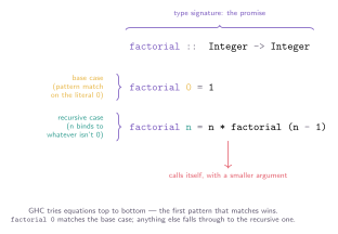
Figure: factorial, taken apart. GHC tries each equation in order, top to bottom, and uses the first one whose pattern matches the actual argument.
Patterns can go well beyond literal numbers — they can take a data structure apart directly:
firstOf :: (a, b) -> a
firstOf (x, _) = x                -- _ means "I don't care about this part"

headOr :: a -> [a] -> a
headOr def []    = def            -- matches the empty list
headOr _   (x:_) = x              -- matches "at least one element"; x is that element

describePoint :: (Int, Int) -> String
describePoint (0, 0) = "origin"
describePoint (0, _) = "on the y-axis"
describePoint (_, 0) = "on the x-axis"
describePoint p@(x, y) = "point " ++ show p ++ " at (" ++ show x ++ "," ++ show y ++ ")"
That last equation uses an as-pattern, p@(x, y): it binds p to the whole tuple while simultaneously taking it apart into x and y — useful whenever you need both the pieces and the original together.
Pattern matching itself traces back to Rod Burstall’s 1969 paper “Proving Properties of Programs by Structural Induction,” which proposed writing cons(a, y) = x instead of a = car(x); y = cdr(x) — taking a structure apart by naming its shape, rather than calling accessor functions on it one piece at a time. Burstall and John Darlington built this into a real language, NPL, in 1977; Burstall, David MacQueen, and Don Sannella extended it into HOPE in 1980, the first language with genuine algebraic data types alongside it. One detail is worth knowing precisely because Haskell chose differently: HOPE’s pattern matching picked whichever clause was most specific, regardless of the order it was written in, while Haskell’s describePoint above uses simple top-to-bottom, first-match-wins order instead — simpler to reason about, at the cost of describePoint (0, 0) silently returning the wrong answer if it were ever accidentally moved below describePoint (0, _). Burstall’s own doctoral students include Conor McBride, co-author of the Applicative Functors paper this book already leaned on in Chapter 10.
describePoint is worth writing in a few other languages, to feel exactly what Haskell’s pattern matching buys for free. C has no tuple type at all, and its own switch matches only integer or enum constants — the closest equivalent is a plain if/else chain testing x and y separately, with no single construct doing the whole job. Java carried the identical limitation for over two decades; only Java 21 (2023) added record patterns, finally letting a switch deconstruct an object’s shape directly (case Point(var x, var y) when x == 0 && y == 0 -> "origin") — decades after Haskell made this the default, unremarkable way to write any function at all. Lisp sits in between: cond branches on arbitrary conditions exactly like a guard, but classic Lisp never destructures automatically — each branch still calls (car p) and (cdr p) by hand to reach inside the pair, exactly the accessor-function style Burstall’s 1969 paper set out to replace in the first place.
Guards: conditions between the pattern and the body
When the choice depends on a condition rather than a shape, a guard reads almost like a mathematician’s piecewise definition:
bmiCategory :: Double -> String
bmiCategory bmi
  | bmi < 18.5 = "underweight"
  | bmi < 25.0 = "normal"
  | bmi < 30.0 = "overweight"
  | otherwise  = "obese"
Each | line is checked top to bottom; the first True guard wins, and otherwise (just True under a friendlier name) catches whatever’s left. Guards and pattern-matched equations combine freely:
classify :: Int -> String
classify n
  | n < 0     = "negative"
  | n == 0    = "zero"
  | even n    = "positive and even"
  | otherwise = "positive and odd"
case expressions: pattern matching mid-expression
Equations put pattern matching at the definition level; case brings the same power inside an expression, anywhere one is needed:
describe' :: Maybe Int -> String
describe' mx = case mx of
  Nothing -> "nothing to see"
  Just 0  -> "exactly zero"
  Just n  -> "got " ++ show n
This is exactly equivalent to writing describe' as separate top-level equations on mx — case is what you reach for when the matching needs to happen partway through a larger function rather than on the whole argument list.
where and let: naming things locally
Both introduce local bindings, visible only nearby — where attaches to a whole set of guarded equations after the fact, let is an ordinary expression you can drop in anywhere:
quadraticRoots :: Double -> Double -> Double -> (Double, Double)
quadraticRoots a b c = (root1, root2)
  where
    discriminant = b*b - 4*a*c
    sqrtDisc     = sqrt discriminant
    root1        = (-b + sqrtDisc) / (2*a)
    root2        = (-b - sqrtDisc) / (2*a)

circleArea :: Double -> Double
circleArea r =
  let piApprox = 3.14159
  in piApprox * r * r
where bindings are shared across all guards of the equation they’re attached to, computed once; let ... in ... is a self-contained expression that can appear anywhere a value is expected, including nested inside another expression.
Currying, partial application, and sections
Chapter 2 goes into why this works from first principles (every Haskell function secretly takes exactly one argument); here’s the practical version. Because f :: a -> b -> c is really a -> (b -> c), supplying only the first argument gives back a perfectly good, reusable function:
add :: Int -> Int -> Int
add x y = x + y

add5 :: Int -> Int
add5 = add 5              -- partial application: supply the first argument, get a function back

ghci> add5 10
15
ghci> map add5 [1,2,3]
[6,7,8]
Sections are the same idea applied to operators, wrapping one side of an infix operator in parentheses to get a one-argument function:
ghci> map (+3) [1,2,3]      -- (+3) means "add 3 to whatever comes in"
[4,5,6]
ghci> map (3-) [1,2,3]      -- (3-) means "subtract whatever comes in, from 3"
[2,1,0]
ghci> filter (>10) [5,15,8,20]
[15,20]
(+3) and Just (+3) show up constantly once you reach Applicatives — (+3) isn’t special syntax tied to Maybe or any other type, it’s just an ordinary one-argument function (Int -> Int, via a section), and Just (+3) is simply that function wrapped in Maybe, exactly the way Just 5 wraps a number. If a section like this ever looks unfamiliar later in the book, it’s worth returning to this paragraph rather than the chapter you’re in — the confusion is almost always about sections, not about whatever new concept is being introduced.
Lambda expressions: functions with no name
Sometimes a function is only needed once, inline, and naming it would be more ceremony than it’s worth — a lambda (Chapter 2’s λ made literal in ASCII as \) creates one on the spot:
ghci> map (\x -> x * x) [1,2,3,4]
[1,4,9,16]
ghci> map (\x -> x `mod` 2 == 0) [1,2,3,4]
[False,True,False,True]
\x -> x * x and a top-level square x = x * x compute exactly the same function — the lambda just never gets a name bound to it, which is fine when it’s only ever used in one place.
Recursion: functions that call themselves
Haskell has no built-in looping construct (for, while) — repetition is expressed as a function calling itself with a smaller version of the problem, exactly as factorial did above:
sumTo :: Int -> Int
sumTo 0 = 0
sumTo n = n + sumTo (n - 1)

length' :: [a] -> Int
length' []     = 0
length' (_:xs) = 1 + length' xs
Every well-behaved recursive function needs two things: a base case that stops the recursion outright (sumTo 0, length' []), and a recursive case that makes real progress toward that base case on every call (n - 1, the shorter list xs). Miss either one and the function either never terminates or never actually computes anything.
Haskell doesn’t lack loops by oversight — recursion (plus the higher-order functions like map and filter you’ve already seen above) is genuinely the only repetition mechanism the language offers, and Chapter 6’s laziness is exactly what keeps this from being a limitation: an infinitely recursive definition like allPositiveIntegers = [1..] is perfectly fine, because nothing forces the recursion to actually finish.
Defining your own types: data, constructors, and newtype
Every type used so far — Int, Bool, [a], tuples — came from the standard library. Pattern matching, guards, and recursion all already work on them fine, which is exactly why this section could wait until now: the data keyword is how you define genuinely new types of your own, and the pattern matching you’ve been writing all chapter is precisely how you’ll take them apart once you do.
data Shape = Circle Double | Rectangle Double Double
  deriving (Show, Eq)
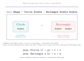
Figure: Shape is the type name. Circle and Rectangle are constructors — functions that build a Shape value, each holding a different number of fields. A value of type Shape is either one or the other, never both: this is why data declarations like this are called sum types.
Constructors are genuinely just functions — Circle :: Double -> Shape and Rectangle :: Double -> Double -> Shape — so building a value looks exactly like an ordinary function call:
myCircle :: Shape
myCircle = Circle 5.0

myRect :: Shape
myRect = Rectangle 3.0 4.0
And pattern matching, which you’ll see everywhere starting in the next section, is precisely how you get the fields back out:
area :: Shape -> Double
area (Circle r)      = pi * r * r
area (Rectangle w h) = w * h
deriving (Show, Eq) asks GHC to automatically generate the boilerplate for converting a value to a printable String (Show) and comparing two values for equality (Eq), rather than you writing that logic by hand. It’s one of the most-used pieces of convenience syntax in everyday Haskell — nearly every data declaration ends with a deriving clause.
Product types: fields held together, not instead of
Rectangle Double Double holds two fields at once — a product type. Combine the two ideas and a data declaration is, in general, a sum of products: a choice of constructors, each bundling together whatever fields it needs.
data Person = Person String Int    -- one constructor, two fields: a product
  deriving Show

data LoginResult = Success Person | Failure String   -- a sum of two cases
  deriving Show
LoginResult reads exactly like the sentence it represents: a login either succeeds, carrying the logged-in Person, or fails, carrying a String explaining why — and the type system won’t let you forget to handle either case.
newtype: a zero-cost wrapper, not a new shape
newtype looks like data restricted to exactly one constructor with exactly one field — because that’s exactly what it is:
newtype UserId = UserId Int
  deriving (Show, Eq)

newtype Email = Email String
  deriving (Show, Eq)
It’s tempting to assume newtype is just data with extra restrictions for no real benefit. The restriction is the entire point: because a newtype can only ever have one constructor wrapping one value, GHC can guarantee it adds zero runtime cost — UserId and Int are represented identically in memory, and the wrapping/unwrapping vanishes entirely during compilation. What you do get, for free, is the type checker refusing to let you pass a raw Int where a UserId was expected, even though they’re indistinguishable once compiled. It’s a compile-time-only safety net, not a data structure.
sendWelcomeEmail :: Email -> IO ()
sendWelcomeEmail (Email addr) = putStrLn ("Welcome email sent to " ++ addr)

-- sendWelcomeEmail (UserId 42)   -- won't compile: UserId isn't an Email,
                                   -- even though both are "really" just Int/String underneath
This pattern — wrapping a primitive type in a newtype purely so the compiler can catch mix-ups — is extremely common in real Haskell codebases: UserId, Email, Age, Meters versus Feet, all wrapping ordinary Ints or Doubles or Strings, precisely so that passing an Age where a UserId was expected becomes a compile error instead of a production incident. Other languages reach for the same idea with names like “branded types” or “opaque types,” usually with far more ceremony than a one-line newtype.
type: a nickname, not a new type at all
Haskell has a third way to introduce a type-looking name, and it’s the one most likely to blindside a newcomer, because it looks almost identical to newtype but behaves completely differently:
type UserId = Int      -- a type ALIAS: just another name for Int
newtype Age  = Age Int  -- a genuinely NEW type wrapping Int
  deriving (Show, Eq)
type does not create a new type at all — it creates a nickname the compiler erases before it ever checks anything. type UserId = Int means UserId and Int are, as far as GHC is concerned, the exact same type, interchangeable everywhere, with zero checking between them:
type UserId = Int
type Age    = Int

getUser :: UserId -> String
getUser uid = "user #" ++ show uid

oops :: Age -> String
oops age = getUser age   -- compiles! Age and UserId are both secretly just Int
This compiles cleanly and silently, because type never introduces anything for the compiler to distinguish — Age, UserId, and Int are one type wearing three labels. Compare this to the newtype Email/UserId example above, where passing the wrong wrapped value was a compile error. If the entire point of introducing UserId was to stop exactly this mix-up, a type alias silently fails at the one job it was asked to do — newtype is what actually delivers on that promise.
So when should you reach for type? Purely for readability, when you have no interest in the compiler enforcing a distinction — most often to give a long, unwieldy type a shorter name:
type ConnectionPool = [(String, Int, Bool)]   -- just a shorter way to write the tuple type

describePool :: ConnectionPool -> String
describePool pool = show (length pool) ++ " connections"
Nobody is likely to accidentally pass a [(String, Int, Bool)] meant for something else into describePool and be glad the compiler stayed quiet about it — here, the alias is pure convenience, not a safety mechanism, which is exactly the case type is for. The rule of thumb: if mixing up two values of the underlying type would be a bug you want caught at compile time, reach for newtype; if you’re just tired of typing out a long type signature, type is the right, lighter-weight tool.
type aliases aren’t limited to simple renames, either — they can take type parameters of their own, exactly like a function takes ordinary arguments, and they can alias a function type just as easily as a data type:
type Validator a = a -> Bool

isEven :: Validator Int
isEven n = n `mod` 2 == 0

isNonEmpty :: Validator String
isNonEmpty s = not (null s)
Validator a isn’t a real type by itself — it’s a pattern for building one, filled in the moment it’s used: Validator Int is nothing more than Int -> Bool, spelled two different ways. isEven :: Validator Int and isEven :: Int -> Bool are, to GHC, the exact same signature; the alias exists purely so a reader sees “this is a validator for Ints” instead of having to reconstruct that meaning from a bare arrow type. This particular pattern — a short, parameterized name standing in for a longer function type — is genuinely one of the most common uses of type in real Haskell code, well beyond the simple UserId-style renames above.
type has one more job later in this book, and it’s worth flagging now so it doesn’t look like a contradiction when it arrives: Type Families’ type family declares a genuine type-level function — something that computes a different type depending on its argument, checked at compile time — which is a considerably more powerful (and more advanced) tool than the plain aliasing this section covers. The shared keyword is not a coincidence; a type family is, in a real sense, what type grows into once it needs to make choices instead of just standing in for one fixed thing.
Modules: how real code is organized
Every code example so far has lived in one imaginary file. Real Haskell projects, obviously, don’t — and the import lines quietly used throughout this chapter (import Data.List, import qualified Data.Map as Map) deserve a proper explanation before going any further.
Every file starts with a module declaration, naming itself and, optionally, exactly what it makes visible to anyone importing it:
-- File: Shapes.hs
module Shapes
  ( Shape(..)   -- export the type AND all its constructors
  , area        -- export just this one function
  ) where

data Shape = Circle Double | Rectangle Double Double

area :: Shape -> Double
area (Circle r)      = pi * r * r
area (Rectangle w h) = w * h

-- perimeter is NOT in the export list above -- invisible outside this module
perimeter :: Shape -> Double
perimeter (Circle r)      = 2 * pi * r
perimeter (Rectangle w h) = 2 * (w + h)
The parenthesized list after the module name is the export list: only Shape (with all its constructors, via (..)) and area are visible to other modules — perimeter, left out on purpose, is a genuinely private helper, exactly as invisible from outside Shapes.hs as a local where binding is from outside its own function. This is Haskell’s actual encapsulation mechanism — not a keyword like private, just an omission from a list.
Importing brings a module’s exports into scope, with a few different styles depending on how much of the imported namespace should be visible directly:
module Main (main) where

import Shapes (Shape(..), area)     -- only these two names, unqualified
import qualified Data.Map as Map     -- everything, but only as Map.foo
import Data.List (sort, nub)         -- an explicit, narrow list
import Data.List hiding (sort)       -- everything except sort

main :: IO ()
main = print (area (Circle 5))
import Shapes (Shape(..), area) brings exactly those two names into scope directly, usable without a prefix. import qualified Data.Map as Map is the pattern this book has used constantly — bringing in everything Data.Map exports, but only reachable through the Map. prefix, which is precisely why Map.insert and a hypothetical unrelated insert from somewhere else never collide. hiding does the opposite of an explicit list: bring in everything except the named exceptions, useful when one specific name from a big module would otherwise clash with something already in scope.
A module’s dotted name isn’t arbitrary — Data.Map genuinely lives at a file path matching that name (Data/Map.hs, inside whichever package provides it), and this convention is enforced by the compiler, not just a style guide. A project’s own modules follow the same rule: a module named MyApp.Database.Users is expected to live at MyApp/Database/Users.hs.
A quick taste of common types
You’ll see these constantly starting in the very next chapter, well before their formal treatment starting in Chapter 9:
-- Maybe: a value, or the honest absence of one
safeDivide :: Int -> Int -> Maybe Int
safeDivide _ 0 = Nothing
safeDivide x y = Just (x `div` y)

-- map, filter, and fold: the three workhorses of list processing
ghci> map (*2) [1,2,3]
[2,4,6]
ghci> filter even [1,2,3,4,5,6]
[2,4,6]
ghci> foldr (+) 0 [1,2,3,4]
10
foldr (+) 0 [1,2,3,4] combines every element with (+), starting from 0, right to left: 1 + (2 + (3 + (4 + 0))). You’ll meet map again, formally, as fmap in Chapter 9 — it isn’t a coincidence that the names rhyme.
Cheat sheet
| Syntax | Meaning |
|---|---|
x :: T | x has type T |
data T = A x | B y z | define a new type T with constructors A, B |
newtype T = T x | a zero-cost wrapper around one field |
type T = U | a nickname for U — no new type, no checking |
f x = ... | define f by equation, matching on x’s shape |
| cond = ... | a guard — checked top to bottom |
case e of ... | pattern match inside an expression |
where ... | local bindings, shared across an equation’s guards |
let ... in ... | local bindings, as a self-contained expression |
f x y | curried application — really (f x) y |
(+3), (3-) | a section — one side of an operator, made into a function |
\x -> ... | a lambda — a function with no name |
f 0 = ...; f n = ... | recursion via base case + recursive case |
Nothing in this chapter is Haskell-specific in spirit — pattern matching, guards, and recursion are just how you’d describe a piecewise mathematical function on paper, transcribed directly into code. That transcription-not-translation relationship between the math and the syntax is precisely this book’s central theme, and Chapter 2 makes the connection formal.
With this vocabulary in hand, every code sample from here on should read as prose, not puzzle — on to Lambda Calculus, where these same shapes turn out to be a 90-year-old idea wearing modern clothing.