Pearls: Beauty in Small Programs
A gallery of short, famous Haskell programs — Quicksort and Mergesort with no swaps or mutation at all, primes tested against the literal textbook definition, a self-building Huffman coding tree, dynamic programming that fills in its own table, and an infinite list of Fibonacci numbers defined in terms of itself — each one a small, complete demonstration of everything this book has covered.
Every field has its “pearls” — short programs so clean they get passed around and taught for decades, each one a complete, self-contained argument for why the language it’s written in exists. This chapter is a small gallery of them, chosen because each one directly showcases an idea from earlier in this book.
FizzBuzz: the smallest pearl
Before the substantial ones, a famous small one — chosen deliberately, because a problem this trivial has nowhere to hide. Any elegance in the solution has to come from the language, not from the problem being secretly hard.
The problem: for every number from 1 to 100, print "Fizz" if it’s divisible by 3, "Buzz" if it’s divisible by 5, "FizzBuzz" if it’s divisible by both, and the number itself otherwise. A standard, unremarkable C solution:
#include <stdio.h>

int main(void) {
    for (int i = 1; i <= 100; i++) {
        if (i % 15 == 0)      printf("FizzBuzz\n");
        else if (i % 3 == 0)  printf("Fizz\n");
        else if (i % 5 == 0)  printf("Buzz\n");
        else                  printf("%d\n", i);
    }
    return 0;
}
Nothing wrong with this — it’s a loop, an if-chain, a print. The straightforward Haskell translation is barely different in spirit, just reshaped into guards:
fizzbuzz :: Int -> String
fizzbuzz n
  | n `mod` 15 == 0 = "FizzBuzz"
  | n `mod` 3  == 0 = "Fizz"
  | n `mod` 5  == 0 = "Buzz"
  | otherwise       = show n

main :: IO ()
main = mapM_ (putStrLn . fizzbuzz) [1..100]
That’s a perfectly good pearl already — but two genuinely different rewrites are worth seeing, each one leaning on a different idea this book has already built up in full.
Gem 1: Monoid, doing the work
Chapter 20 spent an entire chapter justifying <> as “the” way to combine two things of the same type. Maybe’s own Monoid instance — Nothing is the identity, Just a <> Just b combines the insides — turns out to be exactly the shape FizzBuzz needs, if “Fizz” and “Buzz” are treated as optional contributions to combine rather than branches to choose between:
import Control.Monad (guard)
import Data.Maybe (fromMaybe)

fizzbuzz :: Int -> String
fizzbuzz n = fromMaybe (show n) $ mconcat
  [ guard (n `mod` 3 == 0) >> Just "Fizz"
  , guard (n `mod` 5 == 0) >> Just "Buzz"
  ]
guard (n `mod` 3 == 0) is Just () when the condition holds and Nothing otherwise (guard here is Maybe’s own, from Control.Monad); >> Just "Fizz" keeps that “Fizz” only when the guard passed. mconcat then combines the two Maybe Strings with <> — Nothing contributes nothing, and two Justs concatenate their strings — so n = 15 naturally produces Just "Fizz" <> Just "Buzz" = Just "FizzBuzz", with the ordering and the combining both handled by the exact same Monoid instance, not by an explicit branch anywhere in sight. fromMaybe (show n) falls back to the number only when both guards failed and the whole mconcat collapsed to Nothing.
Gem 2: id, as composition’s identity
What IS a Function’s own Chapter 3 proved that (.) and id form a Monoid for functions under composition — id plays exactly mempty’s role. FizzBuzz turns out to be a clean demonstration of that fact in action, treating “Fizz” and “Buzz” as functions that either transform the accumulating string or, via id, do nothing at all:
fizzbuzz :: Int -> String
fizzbuzz n
  | null result = show n
  | otherwise   = result
  where
    result = foldr (.) id
      [ if n `mod` 3 == 0 then ("Fizz" ++) else id
      , if n `mod` 5 == 0 then ("Buzz" ++) else id
      ] ""
Each list element is a function String -> String — either ("Fizz" ++), prepending “Fizz,” or id, changing nothing. foldr (.) id composes the whole list together using exactly the Endo monoid What IS a Function derived — id as the fold’s own starting point is not a coincidence or a placeholder; it is the identity element this composition needs, doing precisely the job mempty does everywhere else in this book. Applied to "", a number divisible by neither leaves both functions as id, the composed result is id "" = "", and null result catches that case to fall back to show n.
Both gems above are really the same trick, told twice: pick a Monoid whose identity naturally means “contributed nothing,” build one small piece per rule, and let <> (or its function-composition cousin, (.)) handle the combining that an if-chain would otherwise have to spell out by hand. FizzBuzz is trivial enough that this is almost showing off — but the identical pattern is exactly how Chapter 23’s HTML combinators and Chapter 20’s mconcat examples scale up to problems that are genuinely not trivial at all.
Quicksort, with no swaps at all
Quicksort, as it’s usually taught, is inseparable from mutation: pick a pivot, walk two indices toward each other swapping elements, partition the array in place. Here is a complete, correct, textbook C++ implementation — the Lomuto partition scheme:
// C++: classic in-place quicksort with explicit index bookkeeping
int partition(std::vector<int>& a, int lo, int hi) {
    int pivot = a[hi];
    int i = lo - 1;
    for (int j = lo; j < hi; j++) {
        if (a[j] < pivot) {
            i++;
            std::swap(a[i], a[j]);       // mutation: two elements swap places
        }
    }
    std::swap(a[i + 1], a[hi]);          // pivot slides into its final spot
    return i + 1;
}

void quicksort(std::vector<int>& a, int lo, int hi) {
    if (lo < hi) {
        int p = partition(a, lo, hi);
        quicksort(a, lo, p - 1);
        quicksort(a, p + 1, hi);          // sort left and right of the pivot
    }
}
Every line of partition is bookkeeping: tracking two indices, deciding when to swap, making sure i and j never trip over each other. It’s efficient — genuinely one of the best general-purpose sorts there is — but reading it tells you almost nothing about why it sorts. You have to trace through the index arithmetic by hand to convince yourself it’s correct.
Now the Haskell version — a direct transcription of quicksort’s actual mathematical definition, from Chapter 5’s insert and this book’s earlier list-comprehension examples:
quicksort :: Ord a => [a] -> [a]
quicksort []     = []
quicksort (p:xs) = quicksort smaller ++ [p] ++ quicksort larger
  where
    smaller = [x | x <- xs, x < p]
    larger  = [x | x <- xs, x >= p]
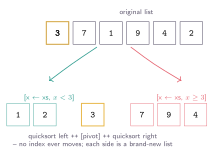
Figure: quicksort (3 : [7,1,9,4,2]) builds two brand-new lists — everything less than 3, and everything not — then recurses on each and glues the three pieces back together with ++. No index ever moves; nothing is ever swapped; every list involved, old and new, coexists unmodified for as long as anything still needs it.
That first split is the whole pattern — the rest of the sort is just that same idea, applied again to each half until nothing is left to split:
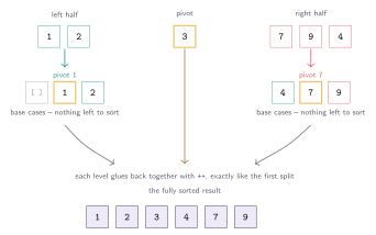
Figure: [1,2] recurses on pivot 1, [7,9,4] recurses on pivot 7 — both bottom out immediately, since an empty list and a single-element list are already sorted by definition, nothing left to prove. Reassembly runs the same ++ glue at every level on the way back up: [] ++ [1] ++ [2] gives [1,2]; [4] ++ [7] ++ [9] gives [4,7,9]; and one last ++ around the original pivot gives [1,2] ++ [3] ++ [4,7,9] = [1,2,3,4,7,9] — sorted.
Read the Haskell version aloud and it is the definition of quicksort: “the sorted list is the sorted smaller elements, then the pivot, then the sorted larger elements.” There is no bookkeeping to trace, because Chapter 5’s immutability means smaller and larger are simply values — computed once, referred to as often as needed, never at risk of the kind of off-by-one error that plagues hand-written partition loops.
This version is not a free lunch on performance: ++ costs time proportional to the length of its left argument, and building two entirely new lists per recursive call allocates far more than the in-place C++ version, which sorts within the original array using only auxiliary stack space. The Haskell version above is a pearl precisely because of its clarity, not because it’s the fastest possible quicksort — Haskell can still get a genuinely in-place quicksort back using the ST monad’s local mutability, once clarity has done its job of proving the algorithm correct.
This exact five-line quicksort, sometimes attributed informally to conversations following Tony Hoare’s original 1960 invention of the algorithm, is one of the most-quoted pieces of Haskell ever written — often used specifically to make the case that functional code can be shorter and more obviously correct than its imperative equivalent, not just different in style.
Mergesort: split, sort, merge
Quicksort partitions around a pivot; mergesort takes an even more direct route to the same goal — split the list in half, sort each half (however that gets done — including, recursively, by more splitting), then merge the two sorted halves back together in order.
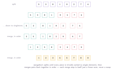
Figure: Split all the way down to single elements — already trivially sorted — then merge pairs back together, in order, all the way back up. Every merge step is a simple linear scan comparing two already-sorted lists; nothing about it needs a pivot, an index, or a swap.
merge :: Ord a => [a] -> [a] -> [a]
merge [] ys = ys
merge xs [] = xs
merge (x:xs) (y:ys)
  | x <= y    = x : merge xs (y:ys)
  | otherwise = y : merge (x:xs) ys

mergeSort :: Ord a => [a] -> [a]
mergeSort []  = []
mergeSort [x] = [x]
mergeSort xs  = merge (mergeSort left) (mergeSort right)
  where
    (left, right) = splitAt (length xs `div` 2) xs
merge is the only place any actual comparing happens, and it reads exactly like the picture: walk both sorted lists side by side, always taking the smaller of the two current heads, until one list runs out — at which point the rest of the other list is already sorted, so it’s simply appended as-is. mergeSort itself does no comparing at all; it just keeps splitting until [] or a singleton (both trivially already sorted), then leans entirely on merge to reassemble the answer.
Mergesort’s worst-case time is , guaranteed — unlike the naive quicksort above, there’s no already-sorted-input pathology to worry about, because mergesort’s split point is always the middle, regardless of what the data looks like. The tradeoff is that a fully persistent, immutable mergesort like this one needs auxiliary space for the merge step, where a well-tuned in-place quicksort can get by with .
Notice the shape of mergeSort itself: two base cases ([] and [x]) and one recursive case that combines the results of two smaller subproblems — the textbook definition of a divide-and-conquer algorithm, transcribed with nothing extra. merge, meanwhile, is doing something you’ll see again shortly: threading through two lists in lockstep, choosing an output at each step, is exactly the shape zipWith uses in the fibs pearl below — just with a comparison instead of a fixed combining function.
Chapter 6 built the infinite list of primes with a sieve — elegant, but the sieving trick (filter out multiples of each prime as you find it) takes a moment of cleverness to see why it works at all. Here is a second, even more literal pearl: primality tested by simply asking the definition of “prime” the question directly.
A number’s factors are exactly the numbers that divide it evenly:
factors :: Int -> [Int]
factors n = [x | x <- [1..n], n `mod` x == 0]

ghci> factors 12
[1,2,3,4,6,12]
ghci> factors 13
[1,13]
A number is prime precisely when its only factors are 1 and itself — which is not a clever trick, it’s the textbook definition, transcribed directly:
isPrime :: Int -> Bool
isPrime n = factors n == [1, n]

primes :: [Int]
primes = filter isPrime allPositiveIntegers
  where
    allPositiveIntegers = [1..]

ghci> take 10 primes
[2,3,5,7,11,13,17,19,23,29]
filter isPrime allPositiveIntegers reads exactly the way you’d say it out loud: “the primes are whichever positive integers are prime.” Chapter 6’s laziness is what makes this legal at all — allPositiveIntegers is a genuinely infinite list, and filter only ever forces as many of its elements as take 10 (or whatever calls it) actually demands, checking isPrime on each candidate one at a time, forever, without needing to know in advance where to stop.
isPrime here recomputes factors n from scratch for every candidate, checking divisibility by every number up to n — work per candidate, compared to the sieve’s much cheaper amortized cost of only checking against primes already found. This version is a pearl for the same reason quicksort was: it is a direct, obviously-correct transcription of the definition, not the fastest way to compute the answer. Reach for this version to state what “prime” means unambiguously; reach for the sieve, or a proper trial-division-with-early-exit, when performance actually matters.
Notice the shape: isPrime doesn’t loop, doesn’t count, doesn’t track a running divisor — it asks a single yes/no question by comparing two lists, factors n and [1, n], for equality. This is the same instinct behind quicksort and Chapter 3’s colourOf: state what the answer is a comparison against, and let list equality and list comprehensions do the rest — math notation with :: instead of , the same correspondence Chapter 2 opened with.
Huffman coding: a binary tree that builds its own alphabet
Data compression sounds like it should demand cleverness; Huffman coding’s actual algorithm is closer to a greedy, almost mechanical recipe — repeatedly merge the two least-frequent symbols into a small binary tree, until only one tree remains. Every symbol’s compressed code is simply the path from the root to its leaf.
import Data.List (sortBy)
import Data.Ord (comparing)
import qualified Data.Map as Map

data HuffTree = Leaf Char Int | Node HuffTree HuffTree Int

weight :: HuffTree -> Int
weight (Leaf _ w)   = w
weight (Node _ _ w) = w

buildTree :: [(Char, Int)] -> HuffTree
buildTree freqs = go (map (\(c, w) -> Leaf c w) freqs)
  where
    go [t] = t
    go ts  = go (Node a b (weight a + weight b) : rest)
      where (a:b:rest) = sortBy (comparing weight) ts
buildTree is the entire algorithm: sort the current trees by weight, merge the two cheapest into one new tree labeled with their combined weight, and repeat — a direct transcription of “always combine the two least-frequent things” with no separate bookkeeping for frequency order at all, since each pass just re-sorts.
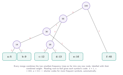
Figure: Six symbols, six starting weights. Each merge picks the two smallest trees so far; the symbol that ends up buried deepest (f, at weight 45, the most frequent) gets the shortest code — a single bit — entirely as a side effect of always merging the cheapest options first.
Reading the codes back out of the finished tree is exactly as direct — walk every path from root to leaf, recording a 0 for every left branch and a 1 for every right one:
codes :: HuffTree -> Map.Map Char String
codes tree = Map.fromList (go tree "")
  where
    go (Leaf c _) prefix   = [(c, if null prefix then "0" else prefix)]
    go (Node l r _) prefix = go l (prefix ++ "0") ++ go r (prefix ++ "1")

encode :: Map.Map Char String -> String -> String
encode table = concatMap (table Map.!)

decode :: HuffTree -> String -> String
decode tree = go tree
  where
    go (Leaf c _) []     = [c]
    go (Leaf c _) bits    = c : go tree bits
    go (Node l r _) (b:bits) = go (if b == '0' then l else r) bits
    go _ []                  = []
decode is the tree walked in reverse: start at the root, follow left or right based on each incoming bit, and every time a Leaf is reached, that’s one decoded character — restart from the root for the next one. Because no code is ever a prefix of another (every symbol lives at a distinct leaf, and leaves never have children), there is never any ambiguity about where one code ends and the next begins.
This buildTree assumes at least two distinct symbols — a single repeated character is a degenerate edge case most real implementations special-case separately, and this pearl doesn’t, in the interest of keeping the core algorithm’s shape visible. Real-world Huffman implementations also don’t re-sort the entire list on every merge; they use a proper priority queue (a min-heap), turning this pearl’s simple-but-quadratic approach into the standard algorithm — the same “clarity first, ST-monad-style optimization once it’s earned its place” tradeoff Quicksort made explicit earlier in this chapter.
Edit distance: a dynamic-programming table that fills itself in
fibs showed self-reference plus laziness acting as memoization for a single sequence. The same trick generalizes cleanly to two dimensions — computing the edit distance between two strings (the fewest single-character insertions, deletions, or substitutions needed to turn one into the other) the classic dynamic-programming way, but with GHC deciding the fill order instead of a programmer:
import Data.Array

editDistance :: String -> String -> Int
editDistance s1 s2 = table ! (m, n)
  where
    m = length s1
    n = length s2
    s1arr = listArray (1, m) s1
    s2arr = listArray (1, n) s2

    table :: Array (Int, Int) Int
    table = array ((0, 0), (m, n))
      [ ((i, j), compute i j) | i <- [0..m], j <- [0..n] ]

    compute 0 j = j
    compute i 0 = i
    compute i j
      | s1arr ! i == s2arr ! j = table ! (i - 1, j - 1)
      | otherwise = 1 + minimum
          [ table ! (i - 1, j), table ! (i, j - 1), table ! (i - 1, j - 1) ]

ghci> editDistance "kitten" "sitting"
3
Look closely at compute: it refers to table, the very array it’s helping define, at strictly smaller indices — (i-1, j), (i, j-1), (i-1, j-1). In an imperative language, this self-reference would demand carefully filling the table in the right order by hand (row by row, or diagonal by diagonal) before any cell could safely read its neighbors. In Haskell, table is simply a value — each cell a thunk that, the moment something asks for table ! (i,j), pulls exactly the neighboring cells it needs and no others, in whatever order they happen to be demanded.
This is Chapter 6’s laziness argument taken to its most striking conclusion: a dependency graph between values (here, a two-dimensional grid of them) resolves itself correctly, with no explicit scheduling, purely because nothing is computed until something else asks for it. The “generate the whole space, let the consumer decide how much to look at” idea that built the infinite list of primes turns out to work identically for a two-dimensional table with genuine internal dependencies, not just a one-directional stream.
Fibonacci, defined in terms of itself
Here is a third, arguably even more startling pearl: the infinite list of Fibonacci numbers, defined by referring to itself:
fibs :: [Integer]
fibs = 0 : 1 : zipWith (+) fibs (tail fibs)

ghci> take 10 fibs
[0,1,1,2,3,5,8,13,21,34]
Read this the way Chapter 6 taught: fibs is a value, not a function call, and Haskell’s laziness means the right-hand side isn’t computed all at once — it’s built exactly as far as something demands. zipWith (+) fibs (tail fibs) pairs each element of fibs with the next element of fibs and adds them — but fibs is the very list being defined, so this only works because laziness lets you refer to a value while it’s still being constructed, consuming each cell only after it already exists.
fibs        = 0 : 1 : 1 : 2 : 3 : 5 : 8 : ...
tail fibs   =     1 : 1 : 2 : 3 : 5 : 8 : ...
zipWith (+) =         1 : 2 : 3 : 5 : 8 : ...   (this becomes fibs, from the 3rd element on)
Every element past the first two is defined as the sum of the two before it — which is exactly the mathematical definition of the Fibonacci sequence, transcribed with no loop, no mutable accumulator, and no explicit recursion on an index at all.
This style — a value defined using itself, made to work by laziness delaying evaluation just long enough — is called corecursion, and it is the natural dual of the ordinary recursion Chapter 4’s length' used. Where recursion breaks a finite problem down into smaller pieces until it bottoms out, corecursion builds a (potentially infinite) structure outward, one lazily-demanded piece at a time. primes from Chapter 6 and fibs here are both corecursive for exactly this reason.
Why these count as “beautiful”
All six pearls share the same shape: each is a direct transcription of the mathematical or logical definition of the problem, rather than a set of instructions for solving it. That gap — between describing what something is and instructing a machine how to compute it step by step — is the gap this entire book has been walking across, one vantage point at a time: immutability (Chapter 5) is what lets smaller and larger be trusted values instead of moving targets; laziness (Chapter 6) is what lets primes, fibs, and editDistance’s table refer to an infinite space, or to themselves, without looping forever; purity (Chapter 7) is what lets you trust that quicksort xs means the same thing everywhere it appears.
Short, self-evidently-correct code isn’t just an academic nicety — it’s a direct productivity and safety argument. Codebases with a strong functional-core discipline (even in otherwise imperative languages, via libraries like Java’s Streams or C++‘s ranges) consistently report fewer off-by-one and state-synchronization bugs in exactly the kind of code these pearls represent: partitioning, filtering, and building sequences.
This is also, deliberately, close to the end of the pilgrimage. Every idea these short programs lean on — types, immutability, laziness, purity, and the Functor/Applicative/Monad vocabulary from the summit — is something you now have a name for. That’s the real payoff of the climb: pearls like these stop looking like tricks, and start looking like the obvious way to write the code.
Haskell in the wild
Every idea in this book has, by now, shown up only in small, self-contained examples — which can leave a fair question hanging: does any of this actually get used? It does, and not just in academic corners.
Pandoc, the universal document converter that can very plausibly have built the PDF or webpage you’re reading this on, is a Haskell library and command-line tool — its clean separation of readers (parsing a format into an abstract syntax tree) from writers (rendering that tree into another format) is a functional-core design almost identical in spirit to the pure-core-versus-IO-shell architecture from Chapter 7.
Xmonad, a tiling window manager used daily by a real, if niche, community of Linux users, is written and configured entirely in Haskell — its original implementation fit in about 500 lines of code, small enough that its own authors credited Haskell’s expressiveness and strong type system for keeping a genuinely useful piece of systems software that compact.
GitHub built Semantic, a tool for parsing, analyzing, and comparing source code across many languages, in Haskell — citing the language’s strengths in exactly the areas this book has spent the most time on: strong typing, laziness, and purity.
Standard Chartered, a multinational bank, runs a large fraction of its wholesale banking and trading infrastructure — reportedly millions of lines of code — on Haskell and an in-house strict dialect of it, specifically because purity and static typing hold up well under the weight of a large, long-lived, high-stakes codebase.
Haskell has an unofficial community motto, coined by Simon Peyton Jones (one of Haskell’s own designers, quoted at the very start of this book): “avoid success at all costs.” It’s a joke — but a real one, meaning roughly that chasing mainstream popularity too early can quietly corrupt a language’s willingness to keep experimenting. Judging by Pandoc, Xmonad, and the production systems above, the language seems to have quietly succeeded anyway.
The pilgrimage continues
This is the summit of this particular trail — but not of the range. If you’ve followed the Further Peaks chapters that follow this one, Optics, Type Families, and Effects Beyond IO have already taken you well past where earlier drafts of this pilgrimage used to stop. Category Theory still has more territory even past that — Monoids, Traversable in full, Arrows, free monads — and full dependent types are the next mountain range over from everything this book calls “advanced.” And the Haskell ecosystem itself — QuickCheck, real production codebases at scale, the wider library landscape beyond what The Toolbox could cover — is its own separate landscape entirely, only glimpsed here.
None of that is a reason to feel like this book left something unfinished. A pilgrimage was always going to end at a summit, not the summit — the view from here is real, and it’s yours now. Simon Peyton Jones, closing a public lecture on the joy of computer science decades into his career, put it simply:
“It is also rich, beautiful, and fun.”
That was true on page one of this climb, and it’s still true here. Go build something.