Common Algorithms and Data Structures
A practical survey tying Pearls' Quicksort and Mergesort to the rest of the sorting landscape, showing why binary search needs the right data structure to actually be fast, and building a binary search tree from scratch before handing off to the real, production-grade Data.Map and Data.Set.
Sorting, compared
Pearls already built two genuinely different sorting algorithms — Quicksort (partition around a pivot) and Mergesort (split, sort halves, merge). A third, simpler than either, rounds out the comparison:
insertionSort :: Ord a => [a] -> [a]
insertionSort = foldr insert []
  where
    insert x []     = [x]
    insert x (y:ys)
      | x <= y      = x : y : ys
      | otherwise   = y : insert x ys

ghci> insertionSort [5,3,8,1]
[1,3,5,8]
insert slides one element into its correct position in an already-sorted list; foldr (Chapter 3) builds the whole sorted list one insertion at a time, right to left. It’s the most direct possible transcription of “keep a sorted pile, slide each new card into place” — genuinely how most people sort a hand of playing cards.
| Algorithm | Best | Average | Worst | Stable? |
|---|---|---|---|---|
| Insertion Sort | yes | |||
| Quicksort (Pearls) | yes* | |||
| Mergesort (Pearls) | yes |
* the list-based Quicksort from Pearls happens to preserve relative order of equal elements; a mutating, in-place Quicksort generally does not.
Mergesort’s worst case never degrades, because its split point is always the midpoint by position (Pearls) — Insertion Sort’s worst case is an already-reverse-sorted list, where every single insertion has to walk all the way to the far end.
Searching: why the data structure matters as much as the algorithm
Linear search needs no ceremony — elem already is linear search, walking the list until it finds a match or runs out, either way. Binary search is the famous improvement — but only if it’s built on the right foundation.
import Data.Array

binarySearch :: Ord a => a -> Array Int a -> Maybe Int
binarySearch target arr = go lo hi
  where
    (lo, hi) = bounds arr
    go l h
      | l > h     = Nothing
      | otherwise =
          let mid    = (l + h) `div` 2
              midVal = arr ! mid
          in case compare target midVal of
               EQ -> Just mid
               LT -> go l (mid - 1)
               GT -> go (mid + 1) h
This binary search is only because Data.Array’s ! is random access. Writing the exact same algorithm over a plain Haskell [a] instead — using !! to index the middle element — is a genuine trap: list indexing is itself , so an -step binary search over a list costs per step, for a real total of — asymptotically worse than a single linear scan. The algorithm’s shape alone doesn’t guarantee its complexity; the data structure underneath has to actually support the access pattern the algorithm assumes.
Trees: building a binary search tree from scratch
A binary search tree (BST) keeps values ordered so that everything in a node’s left subtree is smaller, and everything in its right subtree is larger — the same ordering invariant that makes binary search on an array work, just expressed as a shape instead of a sorted sequence.
data BST a = Leaf | Node (BST a) a (BST a)

insert :: Ord a => a -> BST a -> BST a
insert x Leaf = Node Leaf x Leaf
insert x t@(Node l y r)
  | x < y     = Node (insert x l) y r
  | x > y     = Node l y (insert x r)
  | otherwise = t   -- already present

member :: Ord a => a -> BST a -> Bool
member _ Leaf = False
member x (Node l y r)
  | x < y     = member x l
  | x > y     = member x r
  | otherwise = True

toList :: BST a -> [a]
toList Leaf         = []
toList (Node l x r) = toList l ++ [x] ++ toList r
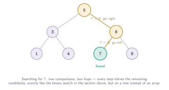
Figure: Two comparisons, two hops, to find 7 in a tree of seven values — the same halving-the-candidates idea as array-based binary search above, expressed as tree structure instead of index arithmetic.
toList’s in-order traversal — left subtree, then the node, then right subtree — always produces a sorted list, for free, as a direct consequence of the insertion invariant; it’s a nice self-check that insert is behaving correctly. insert and member both run in on average, following exactly the halving pattern the figure shows — but only on average.
An unbalanced BST’s worst case is : inserting already-sorted data produces a tree that’s really just a linked list wearing a Node costume, with every element hanging off the right child of the last. Real-world tree-based dictionaries fix this by self-balancing — rotating the tree during insertion (AVL trees, red-black trees, and the size-balanced trees Data.Map actually uses internally) to guarantee height no matter what order values arrive in, not just on average.
Dictionaries and sets: Data.Map and Data.Set
Hand-rolling a BST is the right way to understand an ordered dictionary; Data.Map, from the containers package, is the right way to actually use one — a genuinely balanced, guaranteed- tree, battle-tested, and already in nearly every Haskell project’s dependency tree.
import qualified Data.Map as Map

wordCounts :: [String] -> Map.Map String Int
wordCounts = foldr (\w -> Map.insertWith (+) w 1) Map.empty

ghci> wordCounts ["the","cat","sat","on","the","mat"]
fromList [("cat",1),("mat",1),("on",1),("sat",1),("the",2)]

ghci> Map.lookup "the" (wordCounts ["the","cat","the"])
Just 2
Map.insertWith (+) w 1 reads as “insert w with value 1, or if w is already a key, combine the old and new values with (+)” — the classic word-frequency counter, in one line. Data.Set, from the same package, is the same balanced-tree idea with no attached values at all — conceptually close to a Map k (), used whenever membership alone (not an associated value) is what matters:
import qualified Data.Set as Set

ghci> Set.member 3 (Set.fromList [1,2,3,4])
True
ghci> Set.fromList [1,2,3] `Set.union` Set.fromList [3,4,5]
fromList [1,2,3,4,5]
Data.Map (and Data.Set) are lazy in their values by default — Map.insertWith (+) w 1 builds up exactly the same kind of unevaluated thunk chain Practical Haskell’s tuple trap warned about, if a key is updated many times before anything ever looks at its value. Data.Map.Strict (a drop-in replacement, same API) forces each value to WHNF on every insert, which is almost always what you want for accumulator-style usage like wordCounts above — reach for Data.Map.Strict by default, and the lazy Data.Map specifically when you have a good reason to defer evaluation.
Data.Map and Data.Set are two of the most-imported modules in the entire Haskell ecosystem — configuration lookups, deduplication, frequency counts, graph adjacency lists, and caching all reach for them constantly, precisely because “give me a balanced tree with guaranteed logarithmic operations, already written and already correct” is such a common need that almost nobody hand-rolls their own BST in production code the way this chapter just did for teaching purposes.
The throughline across this whole chapter is the same one Pearls opened with: a naive, obviously-correct version first (insertionSort, a hand-rolled BST), then the real, production-hardened version once the underlying idea is genuinely understood (Data.Map, self-balancing trees, array-backed binary search) — clarity earning its way to performance, never skipping straight to the second half.